Summary of Work for July 1999 (Project #14-08239-F)
Computational Support for the HEU to LEU Conversion of the UMLRR
Dr. John R. White, Justin Byard, and Areeya Jirapongmed
Significant progress was made in several areas during July 1999. The tasks discussed in this Progress Report are as follows:
These tasks are described in further detail in the remainder of this progress report.
Task 1 -- Critical Loading Simulation
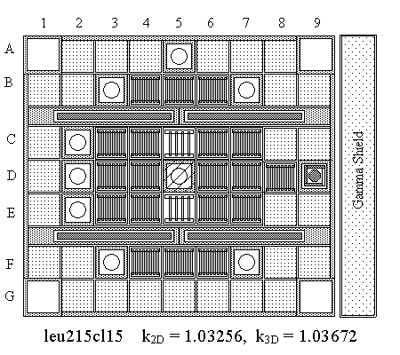
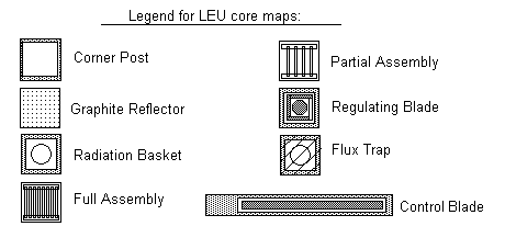
Much of the analysis for this project prior to July 1999 was focused on the selection of a new reference LEU configuration that retains the regulating blade in the D9 location. During June 1999, we finally completed this task, and a 21-element core with 19 full fuel elements and 2 partial elements was chosen as the best candidate for the initial startup of the LEU-fueled UMass-Lowell research reactor (UMLRR). Both 2-D and 3-D VENTURE computational models have been developed and the new reference configurations are referred to as the LEU215 and LEU315 cores, respectively, for the 2-D and 3-D geometries. A top view of the material layout is shown in Fig. 1 along with a legend to help identify the various components for core maps of this type. Several operational parameters for a very similar configuration (LEU214/ LEU314) were tabulated in last month’s progress report, and the reader is referred to the June 1999 Progress report for further details.


Fig. 1 LEU215/LEU315 reference core configuration with legend guide.
With the desired startup configuration known, we turned our attention to the simulation of the initial loading sequence needed to arrive at this end goal. The procedures which describe the steps involved in the critical loading of a new configuration are described in Reactor Operation 1 (RO-1).1 The basic idea is to carefully monitor the subcritical multiplication associated with each new configuration as one goes from only a few elements towards a configuration that leads to a critical system. As the number of fuel elements in the core increases, the subcritical multiplication increases, eventually approaching infinity as a critical configuration is reached.
In monitoring a particular critical loading sequence, one often generates the so-called 1/M line for each step in the sequence. The neutron population and detector count rate is proportional to the neutron source strength and inversely related the degree of subcriticality given by 1-k, where k is the standard neutron multiplication factor. Thus, we can represent the initial count rate for some source-detector configuration as2
![]()
where ![]() is a proportionality constant. If the fuel configuration is changed, possibly by adding additional assemblies at the ith step of a critical loading sequence, eqn. (1) becomes
is a proportionality constant. If the fuel configuration is changed, possibly by adding additional assemblies at the ith step of a critical loading sequence, eqn. (1) becomes
![]()
where ki is the multiplication factor associated with the ith core configuration. The subcritical multiplication for this configuration is defined from the ratio of the current count rate and initial count rate, or
![]()
Substituting eqns. (1) and (2) into the "inverse" of this expression gives
![]()
where ![]() is simply another proportionality constant. The important feature here is that the inverse subcritical multiplication factor, 1/M, is approximately a linear function of the neutron multiplication factor, k. In particular, a plot of 1/M using two known values can be easily extrapolated to the 1/M = 0 point -- which gives a prediction of when the system will be critical (i.e. k = 1).
is simply another proportionality constant. The important feature here is that the inverse subcritical multiplication factor, 1/M, is approximately a linear function of the neutron multiplication factor, k. In particular, a plot of 1/M using two known values can be easily extrapolated to the 1/M = 0 point -- which gives a prediction of when the system will be critical (i.e. k = 1).
Our approach to the numerical simulation of the initial critical loading experiment for the new LEU core involved the computation of the neutron multiplication factor, ki, for several different loading configurations. With this information, a standard 1/M plot could be generated, simulating what might be expected during the actual approach to critical for the new LEU core. The data for the plot were generated with a 2-D VENTURE keff calculation for each of the different assembly configurations. Several 3-D computations were also performed at various stages, but these data were used only to estimate any 2-D versus 3-D differences that might effect our prediction of the critical loading.
The calculations started by loading the core periphery with an arrangement of graphite reflectors and radiation basket assemblies that is consistent with the final proposed LEU215 core configuration as shown in Fig. 1. This arrangement leaves 22 centrally located grid positions available for the placement of full and partial fuel assemblies and the central flux trap irradiation facility.
We decided to initially load only full fuel elements starting in the central core region. New assemblies are then added in a systematic manner, trying to maintain as much symmetry as possible, until the core is nearly critical. At this point, the full fuel assembly in D5 is removed and replaced with the flux trap assembly. In addition, the full fuel elements in C5 and E5 are exchanged with two partial assemblies. Both these moves decrease the core multiplication factor, keff, and increase the inverse subcritical multiplication, 1/M, in the system. After this configuration change, the normal systematic loading of full fuel assemblies is continued until a critical core is reached.
A summary of the actual loading sequence and the data obtained from the VENTURE calculations is given in Table I. Also displayed in Fig. 2 is a visual diary of the core arrangement associated with each step of the simulated loading experiment. Here we see that a sequence of 15 calculations were made, starting with 5 fuel assemblies in the C5, D4, D5, D6, and E5 positions. Two fuel assemblies were added per step for the first several steps and then only one element was added at each step as the system got closer to critical -- and this approach is fully consistent with standard procedures (RO-1) which emphasize a slow careful approach to criticality.
Table I Summary data from the VENTURE critical loading calculations.
|
Case ID |
# of Elements |
Positions Added |
keff (3D) |
keff(2D) |
1/M = (1-k) |
|
cl 1 |
5 |
C5,D4,D5,D6,E5 |
-- |
0.74760 |
0.252 |
|
cl 2 |
7 |
C4,E6 |
-- |
0.82280 |
0.177 |
|
cl 3 |
9 |
C6,E4 |
0.88986 |
0.89152 |
0.108 |
|
cl 4 |
11 |
D3,D7 |
-- |
0.93372 |
0.066 |
|
cl 5 |
13 |
C3,E7 |
-- |
0.96206 |
0.038 |
|
cl 6 |
14 |
C7 |
-- |
0.98134 |
0.019 |
|
cl 7 |
15 |
E3 |
0.99868 |
0.99367 |
0.006 |
|
cl 8 |
14 |
Replace FA with FT in D5 |
-- |
0.95656 |
0.043 |
|
cl 9 |
14 |
Replace FA with PA in C5,E5 |
0.93588 |
0.93309 |
0.067 |
|
cl 10 |
15 |
D8 |
-- |
0.94851 |
0.052 |
|
cl 11 |
16 |
F5 |
-- |
0.96242 |
0.038 |
|
cl 12 |
17 |
B5 |
-- |
0.97476 |
0.025 |
|
cl 13 |
18 |
F6 |
0.99527 |
0.99138 |
0.009 |
|
cl 14 |
19 |
B4 |
1.00687 |
1.00302 |
-0.003 |
|
cl 15 |
21 |
B6, F4 |
1.03672 |
1.03256 |
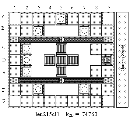
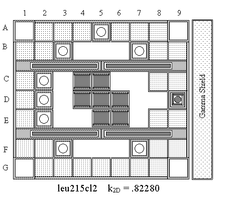
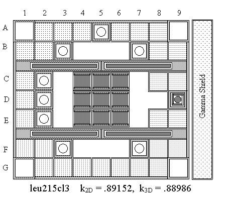
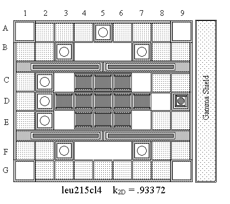
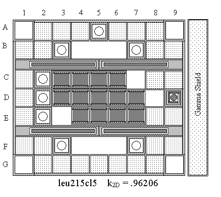
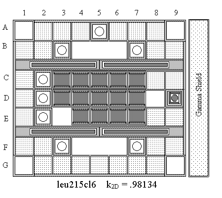
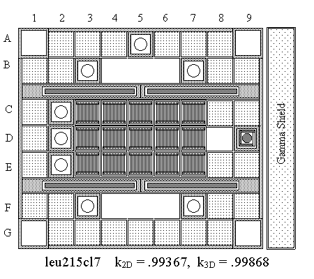
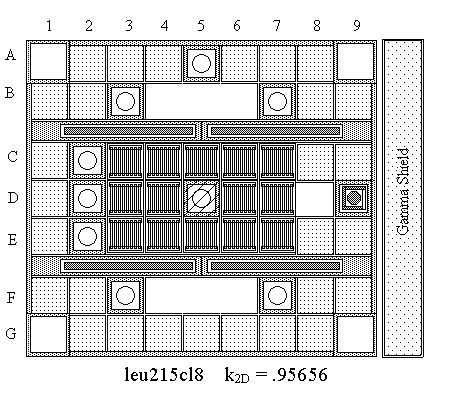
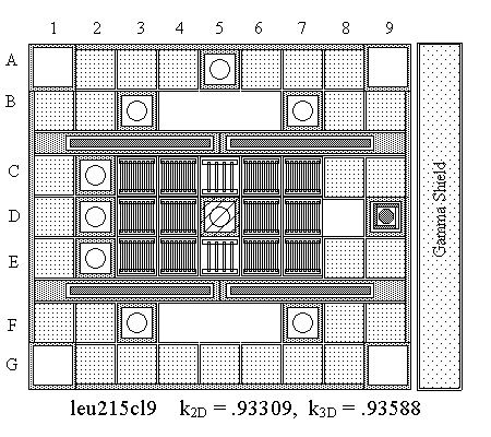
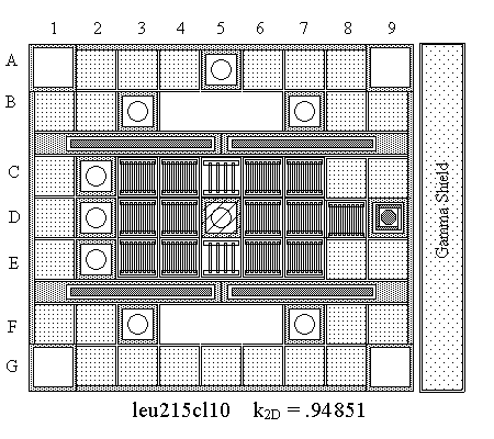
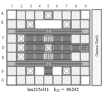
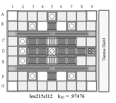
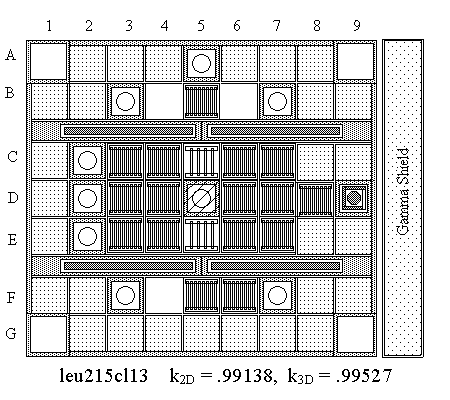
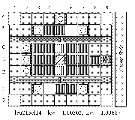
Fig. 2 Core layout at each step of the critical loading sequence.
Note that, at Step 7, 15 full fuel assemblies are loaded into the central 3x5 region of the core. This configuration, with 7 grid positions still containing only water, is nearly critical -- keff from the 3-D calculation is 0.999. Thus, it appears that the critical size of the new LEU fuel assemblies is roughly 15-16 elements with mostly water reflection on the periphery.
However, the final configuration of interest contains a central flux trap facility and two partial assemblies. Thus, at this point, it was decided that Steps 8 and 9 would incorporate these assemblies into the developing core configuration. These modifications decreased reactivity substantially, allowing the critical loading process to continue towards the final desired configuration. After 5 more steps, bringing the total assembly count to 17 full elements and 2 partial elements, the current calculations predict that the system will be slightly supercritical (with no control inserted). Within the limitations of the VENTURE modeling and within the context of the configuration described in Fig. 2, criticality should be reached with about 18-20 elements in the core, with our best estimate showing that criticality is achieved with between 18 and 19 elements loaded (includes two partial elements).
The sequence of 14 steps that lead to a slightly supercritical core is summarized in Table I and in the 14 core configuration maps displayed as part of Fig. 2. These data summarize quite nicely the simulated loading calculations performed here. This simulated experiment was performed to help guide the actual critical loading once the new LEU fuel arrives at UMass-Lowell. During the actual loading, however, the core keff is not directly available to the operators. But, using a ratio of count rates from different configurations, the subcritical multiplication factor in eqn. (3) is easily estimated. With this information, the standard 1/M plot can be used to monitor the loading sequence and predict when criticality will occur.
With the computed keff from the 2-D VENTURE calculations, eqn. (4) with ![]() was used to determine a sequence of 1/M values consistent with the individual steps in the proposed loading scheme. The 1/M values are given in Table I and plotted, along with straight lines that represent linear extrapolations to the 1/M = 0 point, in Fig. 3. This simulated 1/M plot should be very similar to the one actually generated as part of the real critical loading of the LEU-fueled UMLRR. It is easy to see that the system with 15-16 fresh fuel assemblies represents a critical system -- since 1/M approaches zero. Also, it is easy to see the discontinuity that occurs with the interchange of full fuel in D5 and in C5 + E5 with the flux trap and two partial fuel assemblies. After this abrupt increase in 1/M (or decrease in keff), criticality is again approached systematically until a slightly supercritical system is obtained with 19 elements loaded (17 full and 2 partials).
was used to determine a sequence of 1/M values consistent with the individual steps in the proposed loading scheme. The 1/M values are given in Table I and plotted, along with straight lines that represent linear extrapolations to the 1/M = 0 point, in Fig. 3. This simulated 1/M plot should be very similar to the one actually generated as part of the real critical loading of the LEU-fueled UMLRR. It is easy to see that the system with 15-16 fresh fuel assemblies represents a critical system -- since 1/M approaches zero. Also, it is easy to see the discontinuity that occurs with the interchange of full fuel in D5 and in C5 + E5 with the flux trap and two partial fuel assemblies. After this abrupt increase in 1/M (or decrease in keff), criticality is again approached systematically until a slightly supercritical system is obtained with 19 elements loaded (17 full and 2 partials).
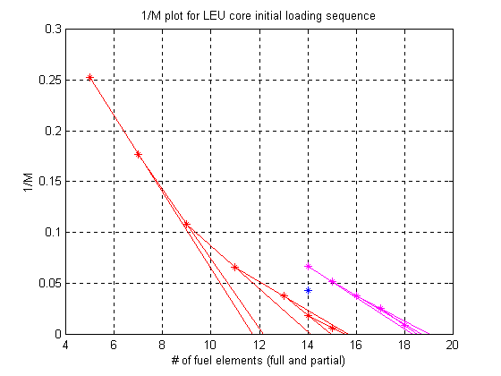
Fig. 3 1/M plot for the proposed initial critical loading sequence.
The final step in the loading procedure adds two additional full fuel assemblies into locations B6 and F4 to obtain the initial startup core for the LEU-fueled UMLRR. This configuration, as shown in Fig. 1, has an excess reactivity of about 3.3 – 3.7![]() based on the 2-D and 3-D VENTURE calculations, respectively. With the 3-D model, the estimated critical blade height needed to offset this excess reactivity is about 16.5 inches withdrawn -- this estimate assumes that the regulating blade is fully out. This configuration, with the blades partially inserted, is expected to be a reasonable approximation to the actual operational configuration for the LEU startup core.
based on the 2-D and 3-D VENTURE calculations, respectively. With the 3-D model, the estimated critical blade height needed to offset this excess reactivity is about 16.5 inches withdrawn -- this estimate assumes that the regulating blade is fully out. This configuration, with the blades partially inserted, is expected to be a reasonable approximation to the actual operational configuration for the LEU startup core.
To summarize briefly, this analysis has identified a candidate sequence of steps that should lead to the desired operating configuration in a systematic predictable manner. The overall plan is broken into two sequences that are separated by a rather large decrease in reactivity when three full assemblies are replaced with the central flux trap and two partial elements. This two-stage procedure was adopted to guarantee a well-behaved 1/M plot over the full range of assemblies loaded. The first sequence predicts criticality with about 15-16 full fuel assemblies and, after reducing the reactivity of the elements in the C5, D5, and E5 positions, criticality is not achieved until 18-19 total elements are loaded. The loading of the two additional full fuel elements gives about 3.5% excess reactivity for normal operation of the facility. This excess reactivity is offset during operation at a just-critical condition by inserting the four large control blades to about 16.5 inches withdrawn. This simulation of the critical loading process, including the data in Table I, the core maps in Fig. 2, and the simulated 1/M plot in Fig. 3, should be an invaluable guide during the actual initial loading of the LEU core.
Task 2 -- Blade #1 Differential and Integral Worth Curves
One of the first tasks that will be required after the LEU initial loading sequence is complete is the calibration of the four large control blades and regulating blade. Differential and integral worth curves are usually generated experimentally via Special Procedure 15 (SP-15) -- Reactivity Worth Calibration.3 This procedure outlines the experimental technique used for gathering the necessary differential reactivity worth data and it suggests that the data be fit to a simple theoretical model given by
![]()
where H represents the full range of the blade in inches (H = 26 inches for the UMLRR) and z gives the blade position in inches withdrawn. This mathematical representation is derived from a very simple bare homogeneous 1-group diffusion theory model of the system. In addition, it assumes that only one control blade is present in the reactor. Equation (5) and its integral lead to the familiar symmetric "bell-shaped" differential blade worth curves and to the symmetric "S-shaped" integral blade worth curves that can be seen in most reactor theory texts.4
Although this simple conceptualization of a typical differential and integral worth curve is an excellent tool for the basic understanding of the physics involved, it was never really intended to be used as a quantitative predictive tool for a real operating reactor. Its biggest drawback is that it gives axially symmetric differential and integral worth curves. In practice, however, this rarely occurs in the UMLRR because the system is operated with the control blades banked at some axial position within the active fuel region. This is required to offset any excess reactivity in the system for operation at a just-critical condition -- as indicated above, the expected critical height for the initial LEU core configuration is 16.5 inches withdrawn. This situation leads to an axially asymmetric neutron flux distribution, with the peak flux occurring below the axial centerline.
The same situation is also encountered when performing blade worth calibrations, in that the remaining three blades are inserted into the core at some position while the worth of the fourth blade is being measured. This is required to maintain the system near critical and it always leads to differential blade worth data that show a bottom-peaked distribution. The problem, of course, is that eqn. (5) cannot model this asymmetry; so the curve fits are never very good.
Although SP-15, with the use of eqn. (5) for the curve fits, has been in use since the startup of the UMLRR, it has been recognized for years that this is probably not the best approach for blade calibration at the UMLRR. With the HEU to LEU fuel conversion planned for late Fall 1999 or early 2000, the time is right to re-evaluate the blade worth calibration procedures to be used for the new LEU core. In fact, the axial region layout within the current 3-D LEU model in the VENTURE code was chosen so that detailed simulations of the blade calibration procedure could be accomplished prior to the startup of the new core.
The focus of the blade worth analyses during July 1999 was geared to Blade #1, but similar calculations are planned for the other control blades and the regulating blade. The LEU315 3-D VENTURE model of the reference 21-element LEU core was used for all the calculations – the only difference among the various runs being the axial location of the control blades (with the regulating blade fixed at the full out position of 26 inches withdrawn). The VENTURE model has 17 axial layers. The top three layers always have control present and the bottom three layers never have control. The middle 11 layers, representing a 26-inch height, vary their control state by simply changing the material composition to contain the homogenized control blade material (control in) or water (control out).
The series of calculations started with Blade #1 fully inserted and Blades #2, 3, and 4 banked at 18.9 inches withdrawn. Since the blades can only be moved in discrete increments consistent with the axial layer thickness in the 3-D VENTURE model, an exact critical state cannot be maintained within the computations. Instead, if keff was within ![]() of unity, we considered this state nearly critical, and appropriate
of unity, we considered this state nearly critical, and appropriate ![]() data for each
data for each ![]() change in the Blade #1 location were recorded. When keff fell outside this bound, Blades #2, 3, and 4 were re-banked to bring the system back to "critical". Using this logic, only one re-bank calculation was needed when Blade #1 was at 14.2 inches out, and the new location of the remaining three blades was 16.5 inches withdrawn.
change in the Blade #1 location were recorded. When keff fell outside this bound, Blades #2, 3, and 4 were re-banked to bring the system back to "critical". Using this logic, only one re-bank calculation was needed when Blade #1 was at 14.2 inches out, and the new location of the remaining three blades was 16.5 inches withdrawn.
Summary data for 13 3-D VENTURE keff calculations are contained in Table II (computations for 12 different Blade #1 positions and a single re-bank calculation). The raw data given in Table II were converted into differential blade worth data in Table III. This table shows the computed ![]() per inch values that are associated with the midpoint of the interval traversed by Blade #1. We have added two zero-worth data points at either end of the blade range, giving N+2 data points for the subsequent fits for the differential worth curves (where N is the number of measured points). The "extra" endpoint data force the mathematical models to be better behaved at the ends.
per inch values that are associated with the midpoint of the interval traversed by Blade #1. We have added two zero-worth data points at either end of the blade range, giving N+2 data points for the subsequent fits for the differential worth curves (where N is the number of measured points). The "extra" endpoint data force the mathematical models to be better behaved at the ends.
Table II Raw data for the simulated differential worth experiments.
|
Position # |
Blade #1 distance withdrawn (inches) |
Blades #2-4 distance withdrawn (inches) |
3-D VENTURE keff |
|
1 |
0.00 |
18.9 |
0.99294 |
|
2 |
1.25 |
18.9 |
0.99308 |
|
3 |
4.18 |
18.9 |
0.99432 |
|
4 |
7.09 |
18.9 |
0.99736 |
|
5 |
9.46 |
18.9 |
1.00116 |
|
6 |
11.8 |
18.9 |
1.00568 |
|
7 |
14.2 |
18.9 |
1.01025 |
|
Re-bank Blades 2-4 |
14.2 |
16.5 |
0.99997 |
|
8 |
16.5 |
16.5 |
1.00388 |
|
9 |
18.9 |
16.5 |
1.00672 |
|
10 |
21.8 |
16.5 |
1.00887 |
|
11 |
24.8 |
16.5 |
1.00986 |
|
12 |
26.0 |
16.5 |
1.00999 |
In an attempt to mimic the actual measurements that are made in the UMLRR, where usually 4-7 actual data values are measured, the data set containing the full 11 ![]() per inch values was filtered into two additional data sets, representing measured data for 7 and 4 actual experimental points. These data, of course, come from the original set of 3-D VENTURE keff computations summarized in Table II, and the data sets with 11, 7, and 4 points are all given in Table III. Thus, we have three sets of simulated data that can be used to test various curve-fitting techniques. As indicated, two zero-worth points are added to each case for the actual curve fits, giving data sets with 13, 9, and 6 experimental points, respectively, for the curve-fitting algorithms. The sets with 7 and 4 measured points are more consistent with actual practice, and the data values in the 11-point set shown in Table III represent an ideal condition. These three data sets will allow verification of the curve-fitting model for data sets with both large and small numbers of experimental points.
per inch values was filtered into two additional data sets, representing measured data for 7 and 4 actual experimental points. These data, of course, come from the original set of 3-D VENTURE keff computations summarized in Table II, and the data sets with 11, 7, and 4 points are all given in Table III. Thus, we have three sets of simulated data that can be used to test various curve-fitting techniques. As indicated, two zero-worth points are added to each case for the actual curve fits, giving data sets with 13, 9, and 6 experimental points, respectively, for the curve-fitting algorithms. The sets with 7 and 4 measured points are more consistent with actual practice, and the data values in the 11-point set shown in Table III represent an ideal condition. These three data sets will allow verification of the curve-fitting model for data sets with both large and small numbers of experimental points.
Table III Simulated differential worth data for Blade #1 in the UMLRR LEU core.
|
Case 1 N = 11 |
Case 2 N = 7 |
||||
|
Point |
Midpoint (inches) |
Worth |
Point |
Midpoint (inches) |
Worth |
|
1 |
0.00 |
0.000 |
1 |
0.00 |
0.000 |
|
2 |
0.63 |
0.011 |
2 |
2.09 |
0.033 |
|
3 |
2.72 |
0.043 |
3 |
5.64 |
0.105 |
|
4 |
5.64 |
0.105 |
4 |
9.46 |
0.177 |
|
5 |
8.28 |
0.161 |
5 |
13.00 |
0.192 |
|
6 |
10.64 |
0.191 |
6 |
16.54 |
0.143 |
|
7 |
13.00 |
0.192 |
7 |
20.36 |
0.073 |
|
8 |
15.36 |
0.166 |
8 |
23.91 |
0.027 |
|
9 |
17.72 |
0.120 |
9 |
26.00 |
0.000 |
|
10 |
20.36 |
0.073 |
|||
|
11 |
23.28 |
0.033 |
Case 3 N = 4 |
||
|
12 |
25.38 |
0.010 |
1 |
0.00 |
0.000 |
|
13 |
26.00 |
0.000 |
2 |
3.55 |
0.063 |
|
3 |
10.64 |
0.182 |
|||
|
4 |
18.00 |
0.117 |
|||
|
5 |
23.91 |
0.027 |
|||
|
6 |
26.00 |
0.000 |
|||
As indicated previously, one aspect of this study was to focus on the goodness of the actual mathematical model used to fit the discrete differential worth data. Clearly, we want to study the existing methodology that uses eqn. (5) to represent the data. Because of the rather awkward symmetry constraint associated with eqn. (5), however, we also decided to try a general cubic polynomial model, which, of course, does not have a formal axial symmetry requirement. Finally, after some trial and error tests with other models, we also decided to use a combination model, which simply sums a cubic polynomial and sinusoid, to see if we could minimize observed weaknesses in the separate models. Thus, three mathematical models were tested as possible candidates for fitting the differential worth data, as follows:
Model A Theoretical Model
![]()
Model B Cubic Polynomial
![]()
Model C Combined Polynomial and Sinusoid
![]()
where H is the maximum blade traverse. Note that the units for differential worth are ![]() per inch, since these are the units used routinely by the UMLRR operations staff. The integral worth versus position,
per inch, since these are the units used routinely by the UMLRR operations staff. The integral worth versus position, ![]() , is also computed, and this is simply calculated by taking the integral of eqns. (5)-(7).
, is also computed, and this is simply calculated by taking the integral of eqns. (5)-(7).
A series of fits using the models given in eqns. (5)-(7) with the differential worth data from Table III were made with the assistance of a short Matlab program called BLADE1W.M. This Matlab script file computes the best set of coefficients for each mathematical model, does some quantitative analysis to indicate the goodness of the fit, and then plots the differential and integral worth curves. A typical set of the resultant differential worth curves is shown in Fig. 4 for the case where N = 11 measured data points. Clearly, of the models tested, the combined model (Model C with the cubic polynomial plus sinusoid) gave the best fit to the simulated worth data. All three models have the expected rough "bell-shaped" behavior, but only Model C was able to retain the "wings" at the ends of the blade and accurately represent the "bottom-peaked" nature of the differential worth profile for Blade #1.
This same observation was made for the other data sets with different N. For example, Fig. 5 shows the case for N = 4, and again we see that the combined model gives a pretty good fit -- even with only a few data points. Thus, it appears that Model C may be a much better choice for use as part of the blade calibration procedure within the UMLRR!
Although Figs. 4 and 5 clearly indicate the superiority of Model C versus the other cases, it is common practice to compute a statistical quantity known as the coefficient of determination (COD) to quantify the goodness of fit. A COD of unity implies a perfect fit of the experimental data to the mathematical model, and when comparing alternate models, the model with the largest COD (closest to unity) usually represents the best model for the given data. The coefficients of determination for the differential worths fits were computed within BLADE1W.M and the results are summarized in Table IV. These data definitely show the same trend that was observed in Figs. 4 and 5, with Model C having the largest COD in all cases.
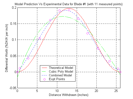
Fig. 4 Differential worth curve fits for Blade #1 with different math models.
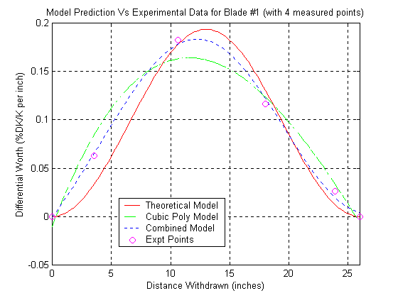
Fig. 5 Differential worth curve fits for Blade #1 with only 4 data points.
Table IV Quality of the fit and the total blade worth for Blade #1.
|
Coefficient of Determination |
Total Blade Worth |
|||||
|
N = 11 |
N = 7 |
N = 4 |
N = 11 |
N = 7 |
N = 4 |
|
|
Model A |
0.958 |
0.955 |
0.951 |
2.57 |
2.57 |
2.52 |
|
Model B |
0.951 |
0.950 |
0.959 |
2.83 |
2.79 |
2.73 |
|
Model C |
0.995 |
0.995 |
0.995 |
2.72 |
2.71 |
2.68 |
Also shown in Table IV is the prediction of the total worth as determined for each of the models with different numbers of experimental data points. These data were obtained from the integral worth curves that are also generated within BLADE1W.M. A sample integral worth curve is shown in Fig. 6 for the N = 11 case, and the total worth of Blade #1 is simply the value of ![]() evaluated at z = H (at 26 inches in Fig. 6). The total worth predicted using Model C falls between the Model A and Model B estimates, and it probably represents a good estimate of the real worth of Blade #1. In addition, the total worth estimate is relatively insensitive to the number of data points used in the curve fits. Thus, the common practice of using 4-7 data points seems quite reasonable.
evaluated at z = H (at 26 inches in Fig. 6). The total worth predicted using Model C falls between the Model A and Model B estimates, and it probably represents a good estimate of the real worth of Blade #1. In addition, the total worth estimate is relatively insensitive to the number of data points used in the curve fits. Thus, the common practice of using 4-7 data points seems quite reasonable.
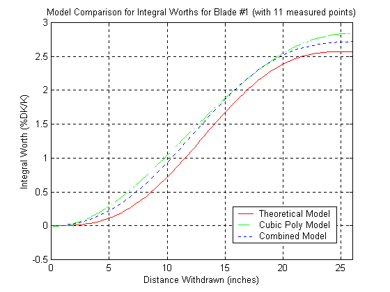
Fig. 6 Typical integral worth curve for Blade #1.
The primary conclusion of this analysis is that the combined model with a cubic polynomial plus sinusoid appears to be the best mathematical model for fitting differential worth data from the UMLRR. The curve-fitting algorithm is relatively easy to implement, and suitable software can be made available for use by the operations staff. A small number of points seem to give good results, so that this part of SP-15 should be left unaltered. Our intent is to perform similar analyses for the other control blades and the regulating blade. If these additional results reflect the same observation as the Blade #1 study, we will strongly recommend an appropriate change to SP-15 to use the new model with a combined cubic polynomial plus sinusoid as the curve-fitting model. The analysis for the other blades should be completed over the next several weeks, and a final recommendation will be made well before the actual conversion of the UMLRR to LEU fuel.
Task 3 -- Development of the 2-D DORT LEU core model
The third major project for July 1999 was the generation of a 2-D DORT model of the LEU core that is fully consistent with the LEU215 VENTURE calculations. Our traditional approach for modeling with the transport theory approximation in DORT is to restrict most analyses to be of the fixed-source type, rather than eigenvalue keff problems. This is the suggested mode of operation because transport theory analyses (in DORT) are generally much more computationally intensive compared to diffusion theory calculations (in VENTURE). However, for fixed-source computations with no upscatter, only one outer iteration is required within the code solution algorithm. Since this represents a significant improvement in runtime relative to eigenvalue or fixed-source problems with upscatter (i.e. problems requiring multiple outer iterations), this mode of operation is definitely the preferred solution scheme. However, since the core physics problem is really an eigenvalue problem, the overall problem solution becomes at least a two-step process -- first we have to compute the fission source, and then this distributed source is used to drive a fixed source transport problem.
In equation form, we can represent the core physics problem as an eigenvalue problem of the form
![]()
where ![]() accounts for the loss and scattering components of the particle balance equation and
accounts for the loss and scattering components of the particle balance equation and ![]() represents the fission source term. The eigenvalue,
represents the fission source term. The eigenvalue, ![]() , is simply the inverse of the multiplication factor
, is simply the inverse of the multiplication factor ![]() .
.
If the fission source term is moved to the right hand side of eqn. (8), then the balance equation can be written as
![]()
For known Q, this expression becomes a fixed-source problem.
The VENTURE code is used to solve eqn. (8) using a few-group diffusion theory approximation. Near the fueled core region, diffusion theory is usually adequate and it gives a good estimate of the eigenvalue and the power distribution within the fueled regions. The neutron source distribution needed for use with eqn. (9) is simply related to the power distribution, as described below.
First let’s denote ![]() as the power density distribution, where
as the power density distribution, where
![]()
where the symbols have their traditional meaning and ![]() gives the average energy release per fission. Now, the multigroup fission source,
gives the average energy release per fission. Now, the multigroup fission source, ![]() , is given by
, is given by
![]()
Combining eqns. (10) and (11) gives
![]()
where the power-to-source conversion factor, ![]() , is given by
, is given by
![]()
For an eigenvalue near unity, ![]() neutrons per fission, and
neutrons per fission, and ![]() MeV per fission, the conversion factor becomes
MeV per fission, the conversion factor becomes ![]() .
.
Thus, the overall strategy for performing the space-energy flux calculations in DORT involves a four-step process:
Several small problem-dependent Matlab and Fortran codes have been written over the last few years to assist in the manipulations involved in Steps 2 and 4, but these codes are not particularly user-friendly and they often require special modifications for each situation of interest. During July 1999, some major modifications and generalizations to the codes that convert the VENTURE power distribution into a distributed source were made. In particular, a Matlab code called PLOT_VPWD was written to plot the VENTURE power distribution and, on option, to write a significant portion of the DORT input file, including the spatial distribution of the fixed source. The PLOT_VPWD code, which is similar to the PLOT_VGEO code that automatically generates large portions of the VENTURE input file (see past Progress Reports), is broken into two main Matlab script files: Plot_Vpwd.m and Write_Dgeo.m. The first part reads the binary power density file from a VENTURE run, and it allows one to view various power distribution profiles through the peak power location. It can also plot 2-D power density surface profiles in any XY, XZ, or YZ plane of interest. The second routine, Write_Dgeo.m, is only called for a 2-D XY model and, if desired, it automatically generates the geometry information (2**, 4**, and 8$$ arrays), material distribution (9$$ array), and the spatial part of the distributed source (96** array) needed for a DORT calculation. The automation of a large portion of the DORT input file has significantly enhanced our ability to perform multigroup coupled neutron-gamma computations for the LEU-fueled UMLRR.
A series of tests were made to validate the new automated PLOT_VPWD code and to explore the basic assumptions involved in the VENTURE-DORT coupling sequence. Our ultimate goal is to produce 47 neutron group and 20 gamma group flux distribution information for the LEU215 configuration. This will allow us to quantify the neutron and gamma radiation environment in the different irradiation facilities in support of various ongoing and future experimental analyses in the UMLRR. However, all the LEU DORT calculations to date were done using an 8-group neutron-only library. The 8-group structure was chosen because consistent 8-group libraries are available for both VENTURE and DORT -- which allows a more direct comparison of results from the various test performed.
In testing the codes and methods, three basic questions needed resolution:
The first two questions are directly related to the validity of the VENTURE-DORT methodology planned for current and future analyses in the LEU-fueled UMLRR. The third question is important because of the difficulty associated with including a DB2 loss term into the DORT analyses. In past studies, this term has simply been ignored, primary because it is not easy to generate the needed DB2 input as a function of group and zone. However, for 2-D models of small cores, the transverse buckling term may indeed be important -- at least in terms of criticality and the overall neutron balance. But, what about the impact of the DB2 loss term on the spatial and spectral distribution of the neutron flux? One of the goals of this series of tests was to answer this latter question. If the transverse buckling does not have a significant effect on the flux distribution, we can simply continue to ignore the DB2 term in DORT, since VENTURE already includes this component in the calculation of reactivity effects. However, if it is important, causing differences in the space and energy flux profiles of ![]() or more, then we certainly will have to deal with this issue in some way.
or more, then we certainly will have to deal with this issue in some way.
Table V summarizes selected results from these studies. Six calculations were performed: two VENTURE keff runs using 2-group and 8-group cross sections, two 8-group DORT fixed-source cases that used the distributed sources generated by PLOT_VPWD with the power distributions from the two VENTURE cases, and two DORT keff cases that differ only in the treatment of the DB2 loss term. The first DORT keff case, D8KNB, has no buckling terms (which is similar to both fixed-source cases) and the second DORT keff calculation, D8KWB, includes appropriate group and zone-dependent DB2 terms; which were generated with data from the 8-group VENTURE calculation.
Zone average fluxes for five zones in the models were tabulated and compared as an illustration of the kind of differences observed for the various cases treated. Table V contains these results, where actual flux data (neutrons/cm2-sec) are given for the VENTURE cases. However, all the DORT results are given as DORT to VENTURE ratios, which represent a measure of the difference in the transport versus diffusion theory results for the 8-group cases.
Table V Methodology verification for various VENTURE-DORT LEU215 calculations.
|
Case Descriptions: |
Zone Descriptions: |
||||||||
|
V2 |
VENTURE 2g keff calc (k = 1.0326) |
Zone 44 |
central fuel region in B5 |
||||||
|
V8 |
VENTURE 8g keff calc (k = 1.0312) |
Zone 55 |
radiation basket center in D2 |
||||||
|
D8V2 |
DORT 8g fixed source calc with V2 source |
Zone 56 |
central fuel region in D3 |
||||||
|
D8V8 |
DORT 8g fixed source calc with V8 source |
Zone 58 |
flux trap center in D5 |
||||||
|
D8KNB |
DORT 8g kcalc with no buckling (k = 1.1453) |
Zone 172 |
top central beamport zone |
||||||
|
D8KWB |
DORT 8g kcalc with DB2 from V8 (k = 1.0465) |
||||||||
|
Group |
V2 |
V8 |
D8V2 |
D8V8 |
D8KNB |
D8KWB |
|||
|
Zone 44 Zone Average Fluxes (n/cm2-s for VENTURE and ratio of DORT to VENTURE for DORT results) |
|||||||||
|
1 |
1.480E+13 |
4.495E+12 |
1.16 |
1.16 |
1.14 |
1.10 |
|||
|
2 |
6.778E+12 |
3.675E+12 |
1.12 |
1.12 |
1.11 |
1.06 |
|||
|
3 |
1.598E+12 |
1.10 |
1.11 |
1.09 |
1.04 |
||||
|
4 |
1.150E+12 |
1.10 |
1.10 |
1.09 |
1.03 |
||||
|
5 |
1.261E+12 |
1.09 |
1.10 |
1.08 |
1.02 |
||||
|
6 |
1.087E+12 |
1.09 |
1.10 |
1.08 |
1.01 |
||||
|
7 |
1.147E+12 |
1.09 |
1.10 |
1.09 |
1.01 |
||||
|
8 |
6.786E+12 |
1.10 |
1.10 |
1.09 |
1.00 |
||||
|
Zone 55 Zone Average Fluxes (n/cm2-s for VENTURE and ratio of DORT to VENTURE for DORT results) |
|||||||||
|
1 |
5.758E+12 |
1.514E+12 |
0.88 |
0.87 |
0.84 |
0.78 |
|||
|
2 |
1.039E+13 |
1.241E+12 |
0.94 |
0.93 |
0.89 |
0.84 |
|||
|
3 |
6.290E+11 |
0.98 |
0.96 |
0.93 |
0.87 |
||||
|
4 |
4.905E+11 |
1.00 |
0.99 |
0.95 |
0.89 |
||||
|
5 |
5.744E+11 |
1.02 |
1.00 |
0.97 |
0.90 |
||||
|
6 |
5.279E+11 |
1.03 |
1.02 |
0.98 |
0.91 |
||||
|
7 |
5.875E+11 |
1.04 |
1.03 |
0.99 |
0.92 |
||||
|
8 |
1.047E+13 |
1.11 |
1.09 |
1.06 |
0.95 |
||||
|
Zone 56 Zone Average Fluxes (n/cm2-s for VENTURE and ratio of DORT to VENTURE for DORT results) |
|||||||||
|
1 |
1.767E+13 |
5.371E+12 |
1.14 |
1.12 |
1.08 |
1.06 |
|||
|
2 |
7.095E+12 |
4.397E+12 |
1.12 |
1.10 |
1.07 |
1.04 |
|||
|
3 |
1.922E+12 |
1.12 |
1.10 |
1.06 |
1.03 |
||||
|
4 |
1.382E+12 |
1.11 |
1.10 |
1.06 |
1.02 |
||||
|
5 |
1.509E+12 |
1.11 |
1.10 |
1.07 |
1.02 |
||||
|
6 |
1.293E+12 |
1.11 |
1.10 |
1.07 |
1.01 |
||||
|
7 |
1.354E+12 |
1.11 |
1.10 |
1.07 |
1.01 |
||||
|
8 |
6.891E+12 |
1.10 |
1.09 |
1.06 |
0.99 |
||||
|
Zone 58 Zone Average Fluxes (n/cm2-s for VENTURE and ratio of DORT to VENTURE for DORT results) |
|||||||||
|
1 |
2.151E+13 |
6.216E+12 |
0.90 |
0.90 |
0.91 |
0.86 |
|||
|
2 |
1.913E+13 |
5.274E+12 |
0.98 |
0.98 |
0.98 |
0.93 |
|||
|
3 |
2.605E+12 |
1.03 |
1.03 |
1.03 |
0.98 |
||||
|
4 |
1.952E+12 |
1.05 |
1.05 |
1.06 |
1.00 |
||||
|
5 |
2.193E+12 |
1.07 |
1.07 |
1.07 |
1.01 |
||||
|
6 |
1.937E+12 |
1.08 |
1.08 |
1.09 |
1.02 |
||||
|
7 |
2.066E+12 |
1.09 |
1.10 |
1.10 |
1.02 |
||||
|
8 |
1.888E+13 |
1.17 |
1.17 |
1.17 |
1.07 |
||||
|
Zone 172 Zone Average Fluxes (n/cm2-s for VENTURE and ratio of DORT to VENTURE for DORT results) |
|||||||||
|
1 |
1.288E+12 |
2.968E+11 |
1.19 |
1.19 |
1.17 |
0.91 |
|||
|
2 |
3.368E+12 |
2.512E+11 |
1.20 |
1.20 |
1.18 |
0.92 |
|||
|
3 |
1.367E+11 |
1.20 |
1.19 |
1.18 |
0.92 |
||||
|
4 |
1.147E+11 |
1.19 |
1.19 |
1.17 |
0.92 |
||||
|
5 |
1.402E+11 |
1.20 |
1.20 |
1.19 |
0.93 |
||||
|
6 |
1.329E+11 |
1.22 |
1.21 |
1.20 |
0.93 |
||||
|
7 |
1.519E+11 |
1.23 |
1.23 |
1.21 |
0.94 |
||||
|
8 |
3.546E+12 |
1.35 |
1.35 |
1.33 |
0.95 |
||||
Several important observations can be made from the information contained in Table V:
Future Work
The two key incomplete issues mentioned above, further computations for the blade worth calibration study and additional verification and analyses with the 2-D DORT model for the LEU215 core, will be the primary focus of work in the coming weeks. Another area, the development of some post processing and plotting capability for the VENTURE and DORT flux files, is also very important. This is essential if we hope to get full benefit from the large amount of information that results from the numerical simulation capabilities in VENTURE and DORT. However, the limited time and resources remaining for this project will limit the amount of effort that can be devoted to this development task. Hopefully some limited capability can be developed before this project comes to closure at the end of next month.
References